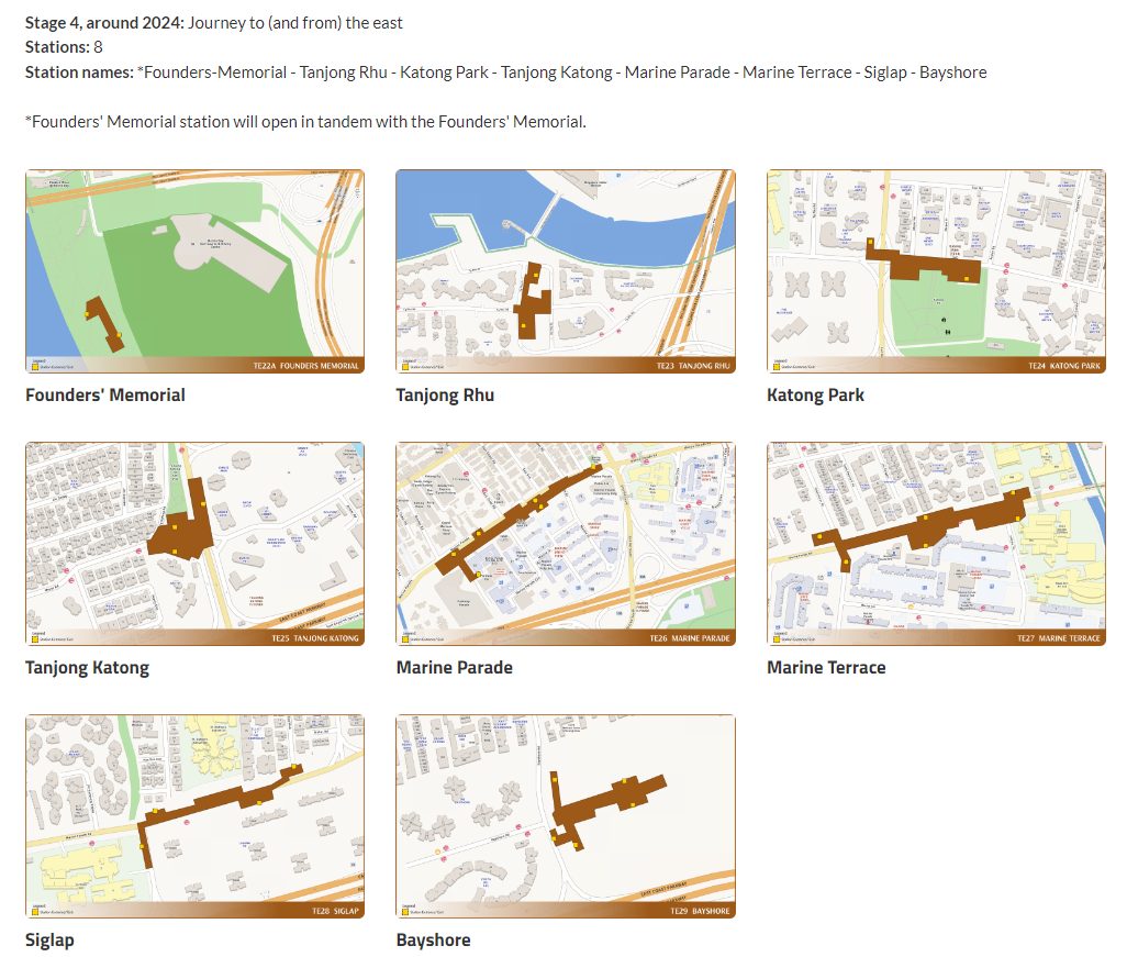
Methodology
Steps taken
Extracting the TEL Stage 4 MRT stations from the Master Plan 2019 Rail Station layer.
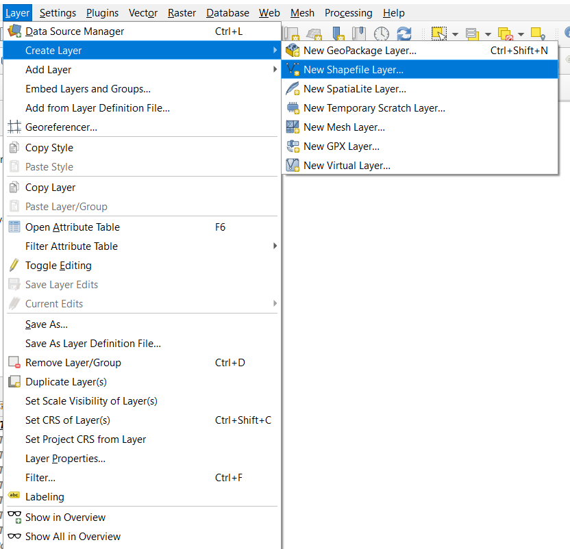
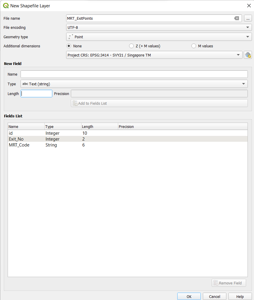
Creating new shapefile layer to map out the location of MRT exits of the new Thomson-East Coast line MRT stations
Extracting out the walkways and pathways people can take.
Using “Iso-area as polygon” function to delineate the catchment area around these MRT stations.
Classify the areas based on 5 minutes, 10 minutes, 15 minutes and 20 minutes walks, based on a walking speed of 4.44 km/h.
Identify the current & projected land use of the catchment areas by analysing the Master Plan 2019 Land Use layer.
Generated the centroids of the OpenStreetMap buildings layer in order to select the buildings that are within the iso-areas using the ‘Select by location’ function. By selecting these centroids, we are able to select the actual buildings that are within the iso-areas.
Identify the types of buildings by analysing the OpenStreetMap buildings layer.
Identify the places of interest in the catchment area by analysing the OpenStreetMap POIS layer, and selecting those within the iso-areas using the ‘Select by location’ function.
Labelling the POIS with SVG symbols, based on the type of POIS.
Standardising the symbologies for different layers.
For cycling path analyses, classifying the iso-areas based on 5 minutes & 10 minutes cycling time from the MRT stations, based on a cycling speed of 16 km/h.
Datasets Used
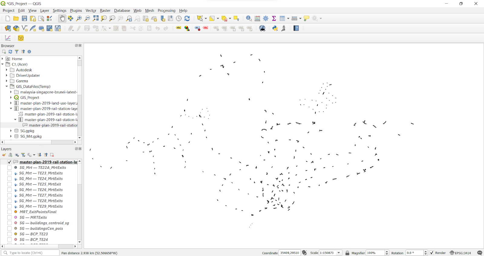
Master Plan 2019 Rail Station Layer from data.gov.sg. This dataset gives us the locations of the MRT stations that are estimated to be done by 2023.
Master Plan 2019 Land Use from data.gov.sg. This dataset shows the projected land use of Singapore until 2023.
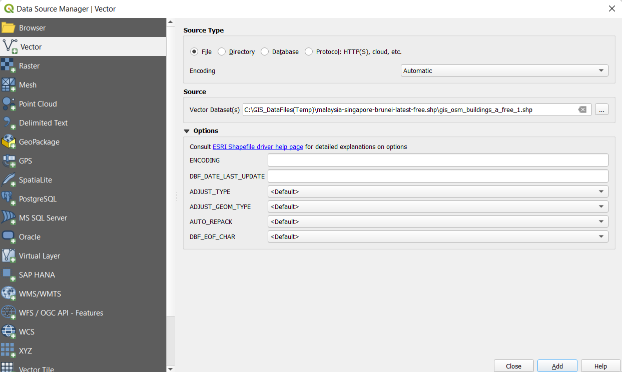
Roads, buildings and places of interest data (labelled as POIS) from OpenStreetMap (OSM) data sets, downloaded from Malaysia, Singapore, and Brunei which is located in the Geofabrik download server.
Extracting the required MRT stations
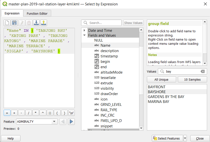
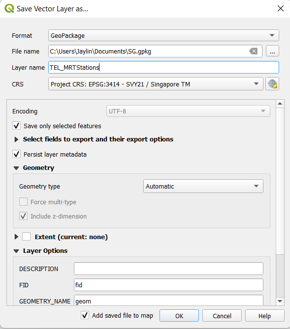
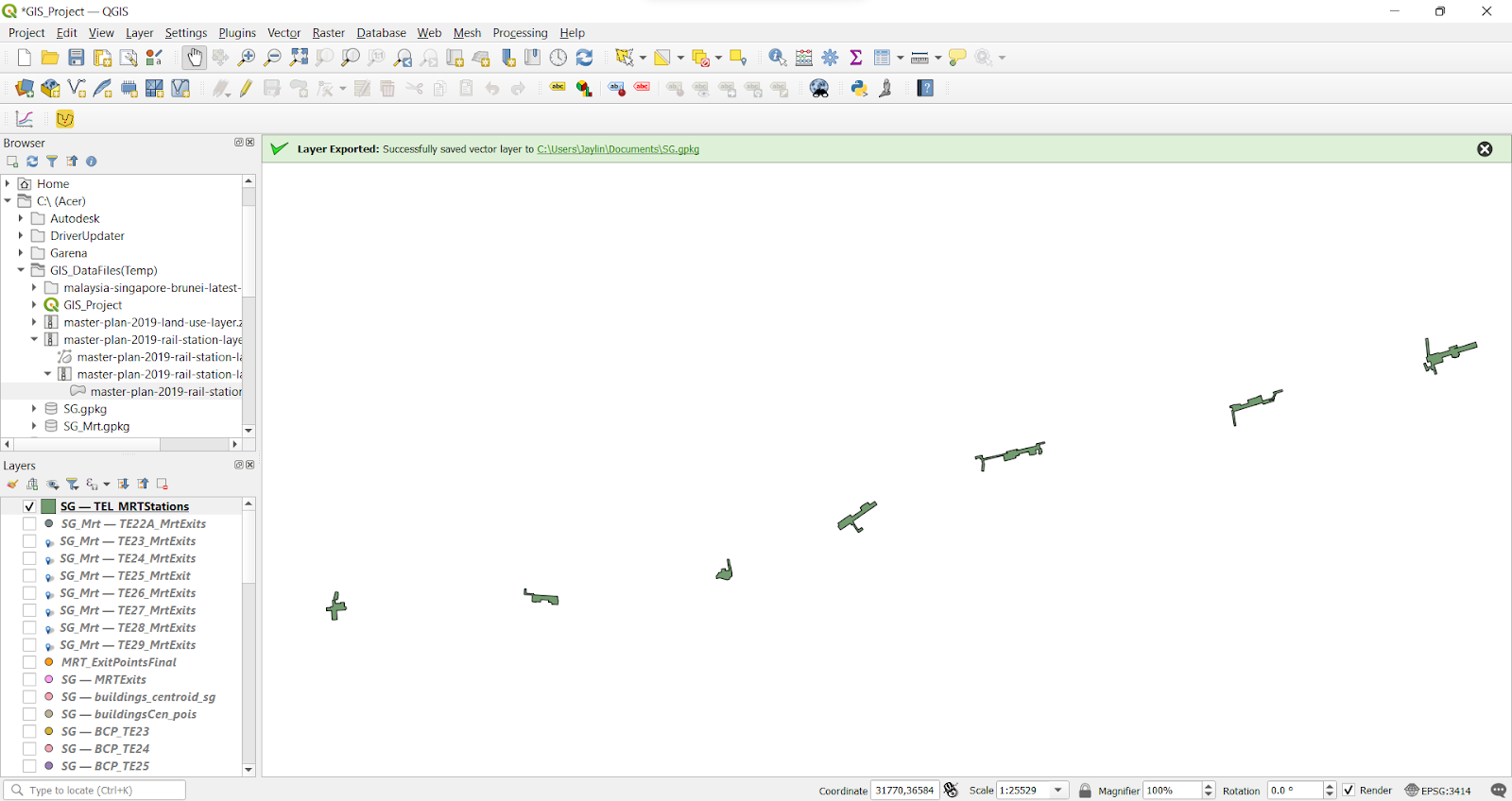
Using the data we have retrieved from data.gov.sg, we were able to obtain the shapefile for the MRT stations (existing and future stations). Using the Select features function, we filtered out only the 7 MRT stations of the Thomson-East Coast line that we will be analysing. All the selected stations were saved into a Geopackage, TEL_MRTStations.
Using the Select by Expression function, we selected out only the 7 MRT stations we want to analyse.
After selecting the MRT stations, we saved these features into a Geopackage.
Locating MRT exits
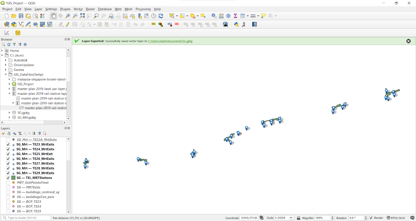
The first step we did was to map out the MRT station exits. This data could not be found online. The only dataset that was provided on data.gov.sg was the Master Plan 2019 Rail Station layer, which showed the indicative MRT station outlines. However, we felt that the outlines were not enough to give us accurate results since one MRT station can have up to five different exits which may serve very different purposes. Hence, by creating a new shapefile, we toggled editing and marked out the location of the MRT exits. We referenced lta.gov.sg to obtain the location of the exits of each station. We then created new shapefile layers of point geometry type and toggled editing to add in the point features where the MRT exits are located.
The screenshots below show the steps we took to create a new shapefile.


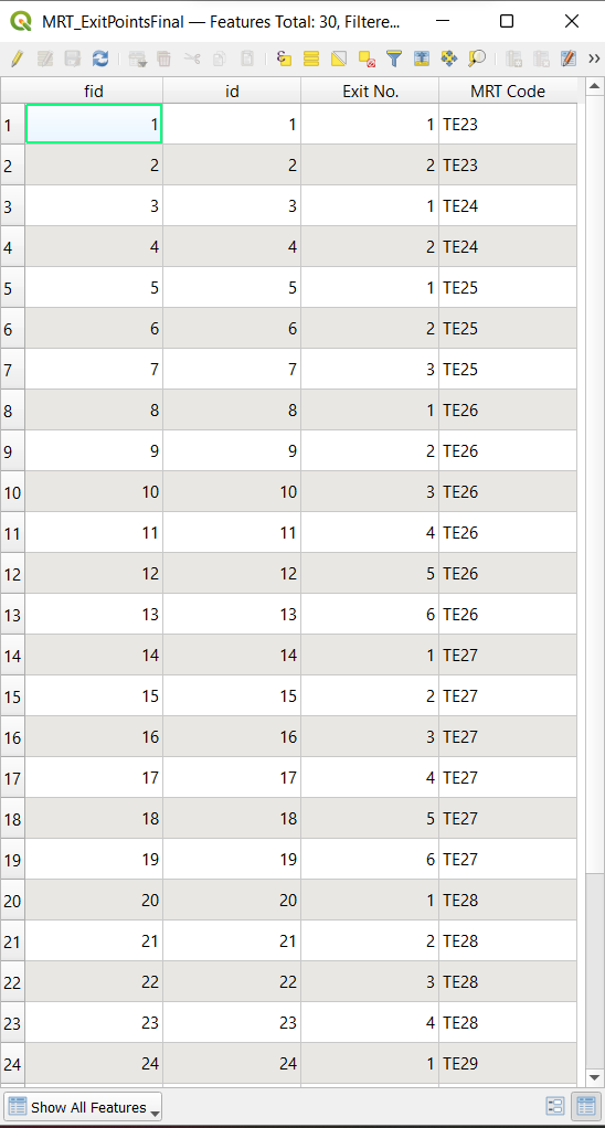
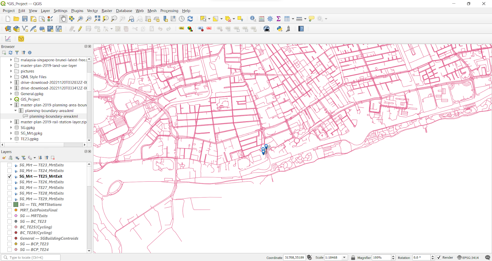
Afterwards, we separated the MRT exits into their own Geopackages by using the Select features by polygon function to pick out the exits for each MRT station. We wanted a separate shapefile for each MRT station since we wanted to analyse each station individually so that there is clear distinction between the Iso-Areas of each station.
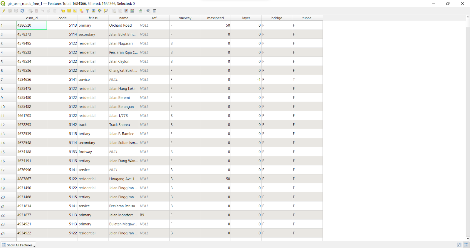
Extracting relevant roads from OSM Roads layer
Since our project only focuses on the immediate catchment area of each station, we were only concerned with the areas within 20 minutes of walking distance. Hence, we extracted all the roads that allowed users to walk on. We had to exclude expressways by filtering out Motorway, Motorway Links, Truckway and Truckway links. After extracting out the roads, we created a new layer to form our network layer and ensure all the roads we linked.
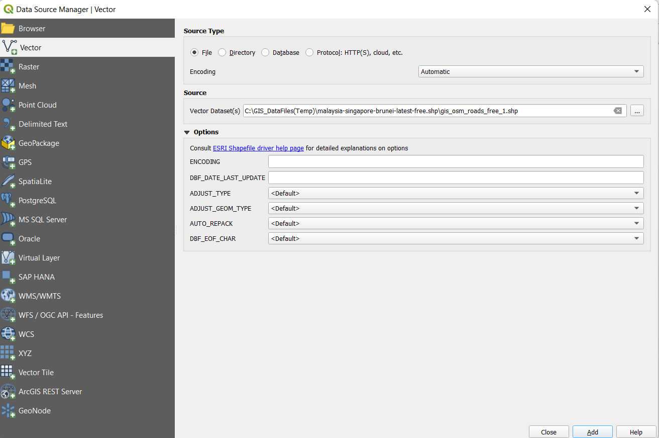
Select the osm_roads_free_1.shp from your file
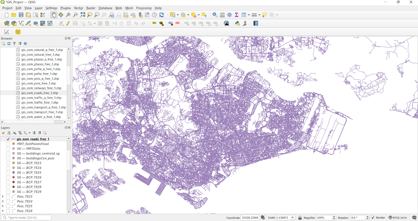

After the layer is loaded, select “select Features by Polygon” from the header.
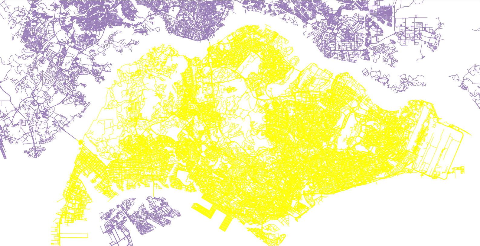
Crop out the designated area of Singapore, to reduce processing power.
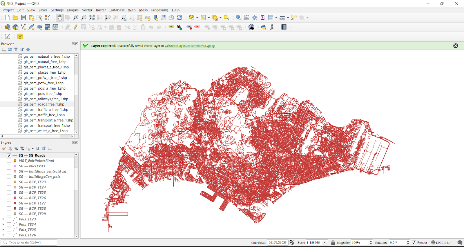
Save the layer in a Geopackage named SG Roads.
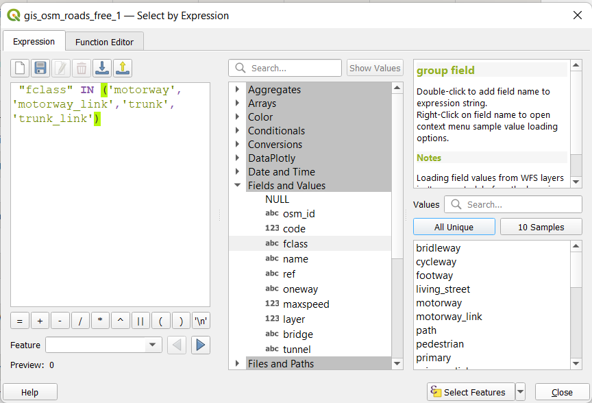
Using the expression above, we selected motorway, motorway_link, trunk and trunk_link from osm roads (which are expressways), which are the paths that pedestrians cannot walk on.
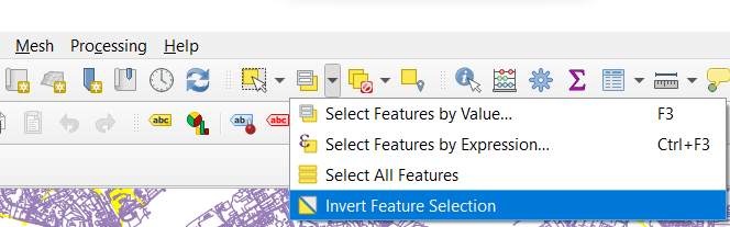
We proceeded to invert the features selected from above. The remaining paths will form the roads with walking paths available, thus making it an important aspect of our catchment area study.
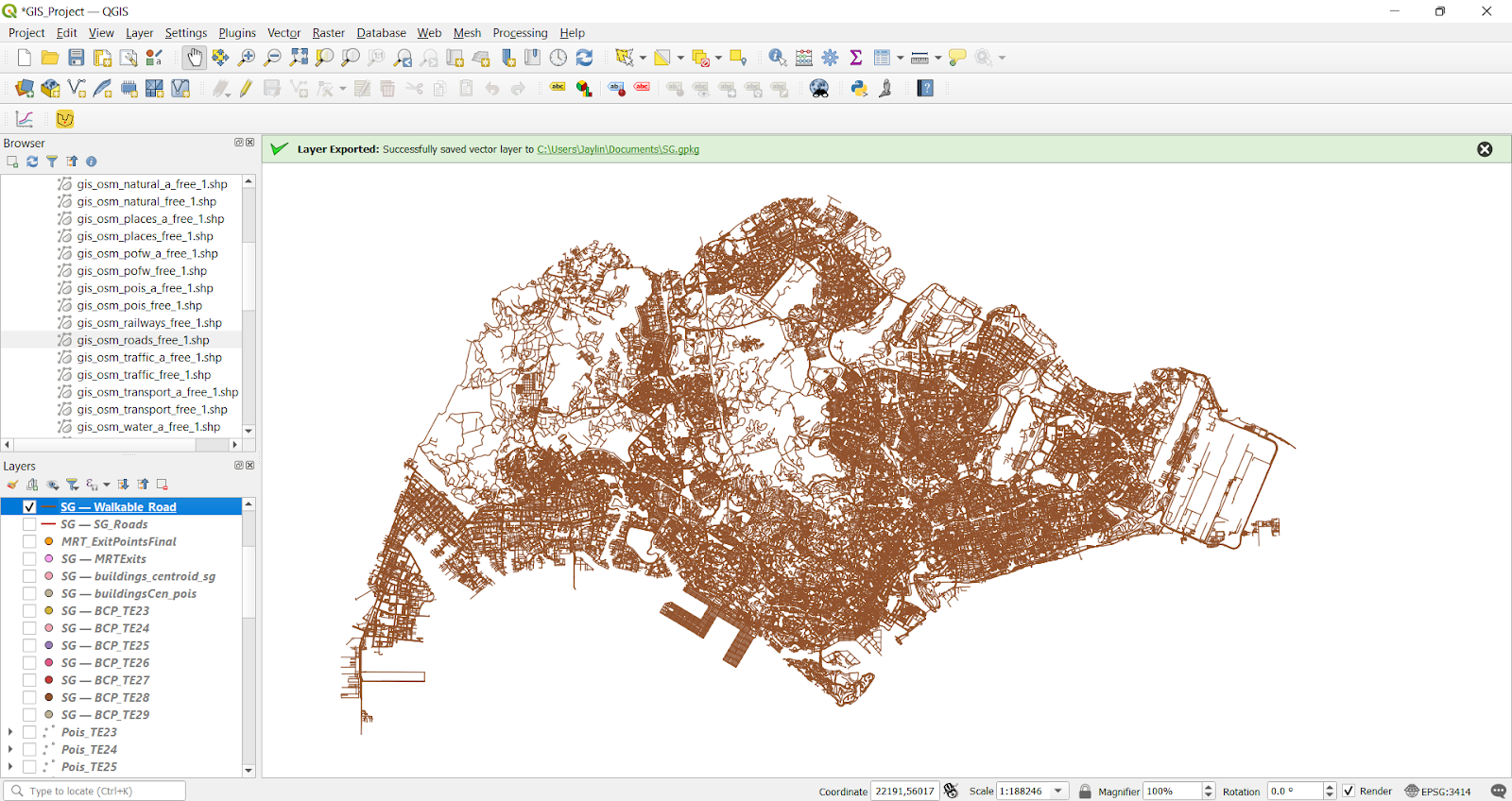
Screenshot above shows all the walking paths in Singapore that are applicable to our study.
Creating Iso-area as polygon layers & classifying the areas based on 5 minutes, 10 minutes, 15 minutes and 20 minutes walk
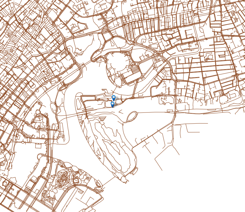
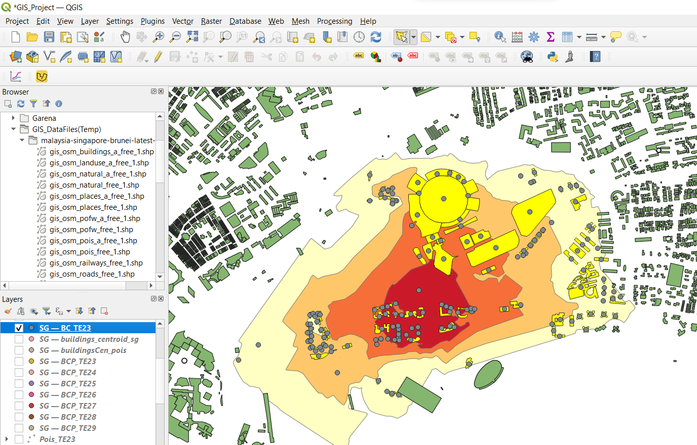
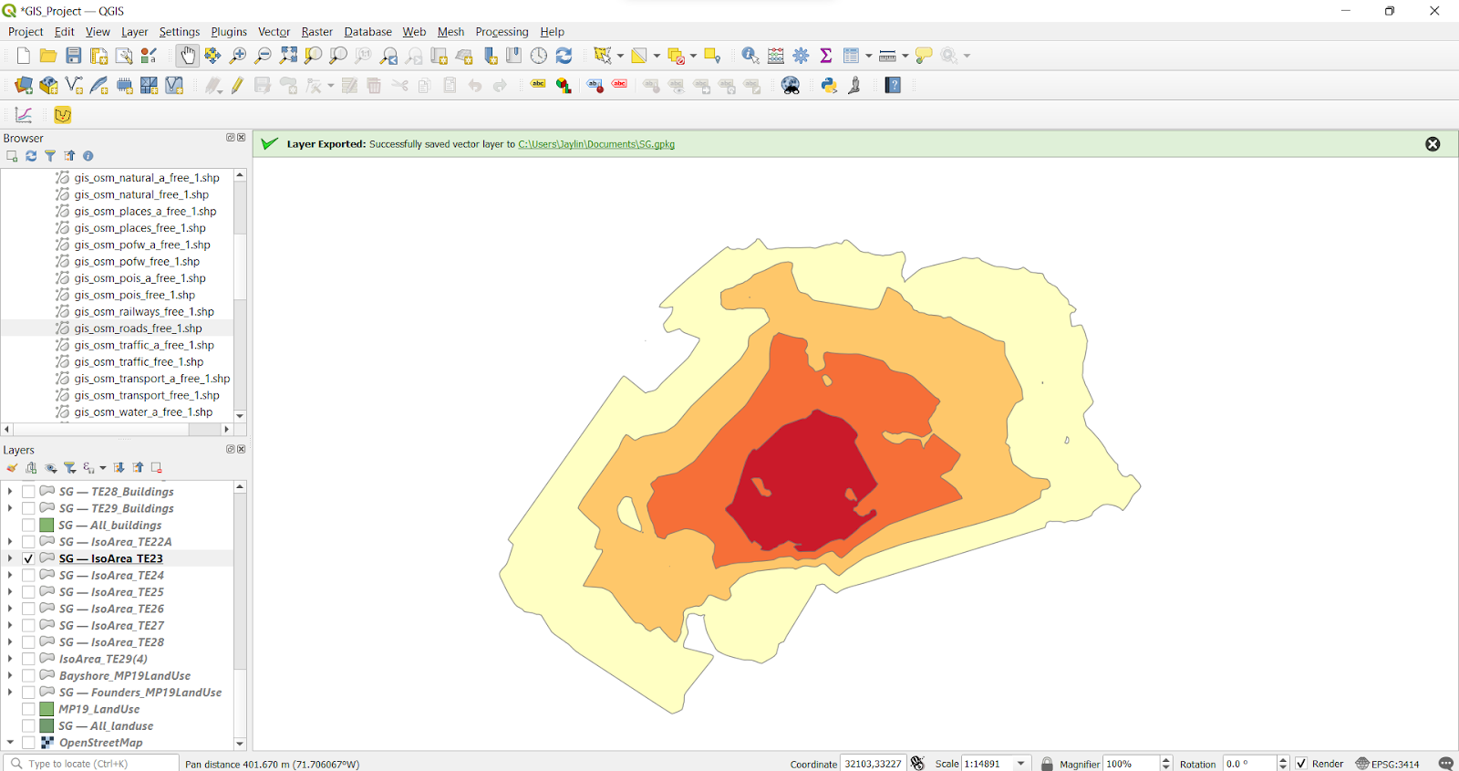
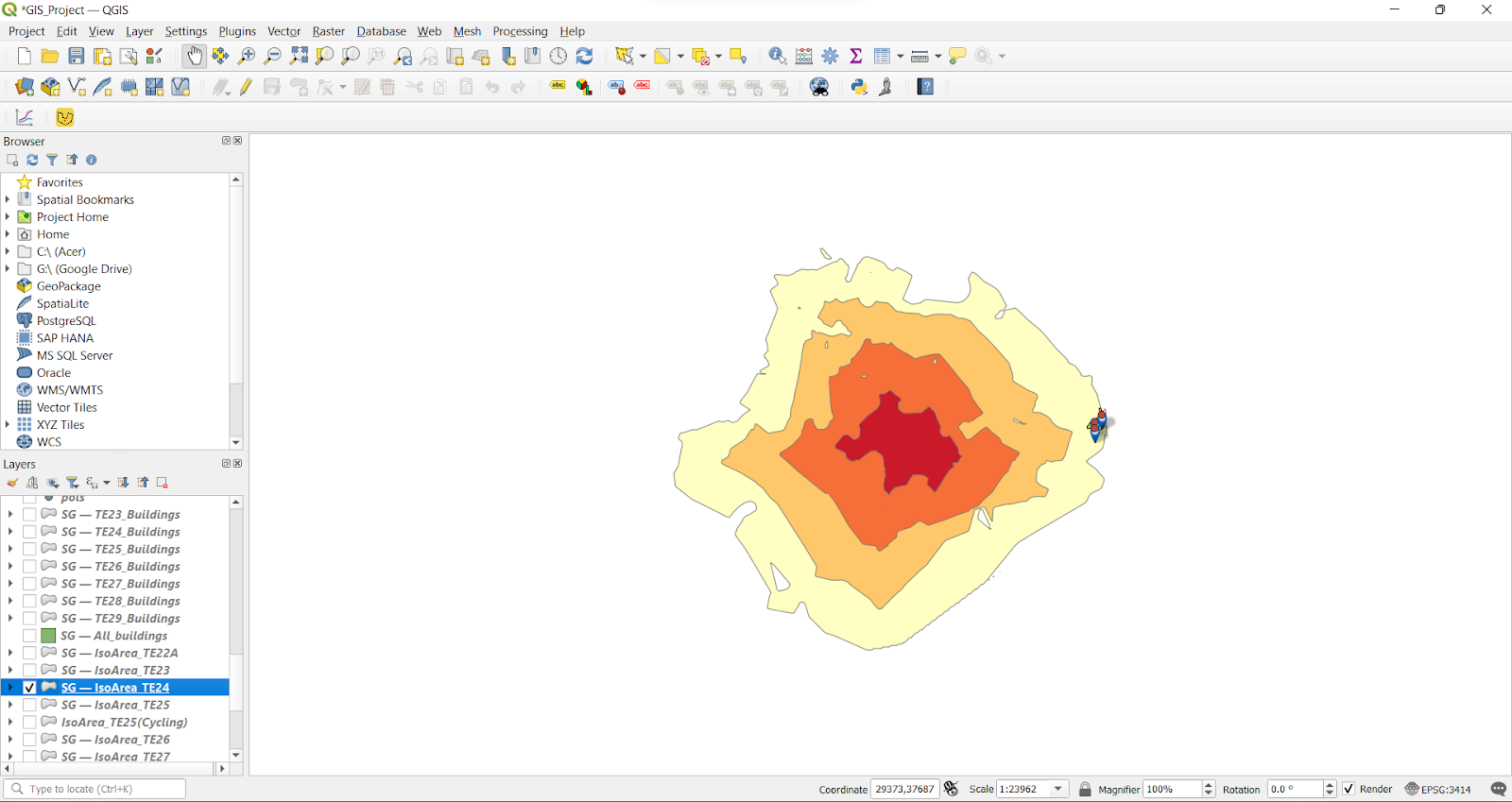
In this example, we will use TE23 (Tanjong Rhu) MRT station as an example for the methods used to generate iso-areas. The blue pointers indicate the exit points of the station and the lines surrounding it indicate the walking paths.
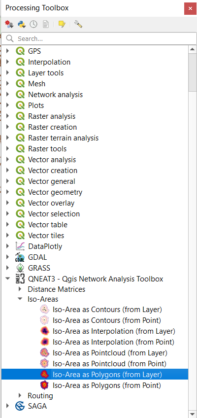
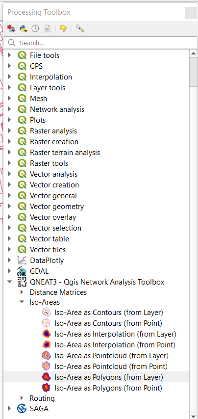
Go to Processing toolbox -> QNEAT 3 -> select Iso-Area as Polygons (from layer).
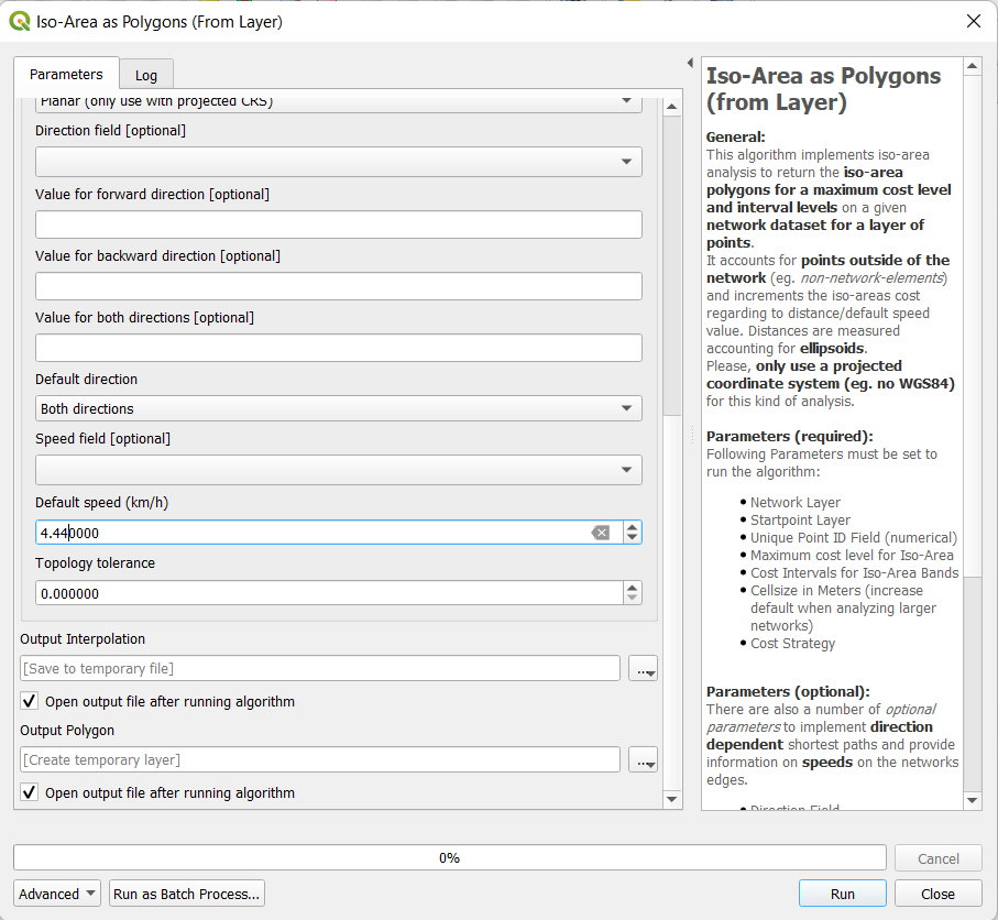
Steps taken in the screenshots above:
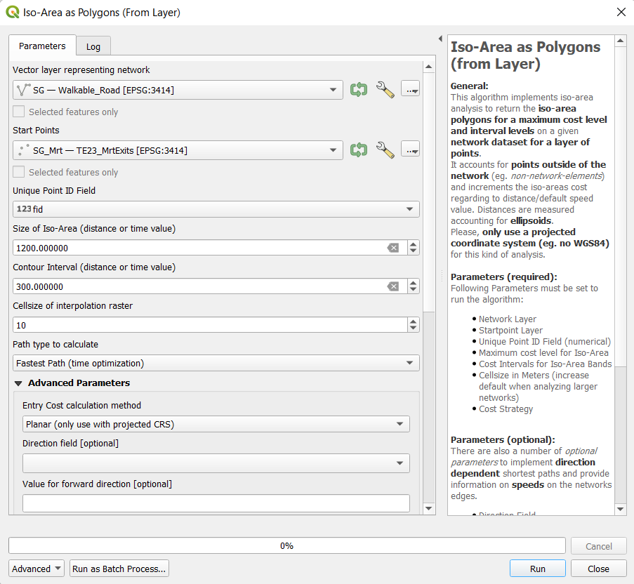
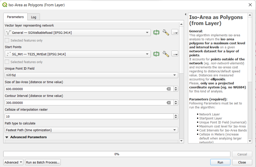
Selecting the paths that are walkable in the Vector layer representing network, which is labelled as Walkable_Road in our project.
Start Points: Selecting the exit points of the MRT station, which is labelled as TE23_MrtExits.
Size of Iso-Area: Time-based. For this project, we are study walking times of up to 20 minutes, which is equal to 1200 seconds.
Contour Interval: Time-based. For the purpose of our analysis, we are using time intervals of 5 mins, which is equal to 300 seconds.
Path type to calculate: Fastest Path (time optimization).
Setting the Default Speed as 4.44km/h, which is the average walking speed that we found in our literature review.
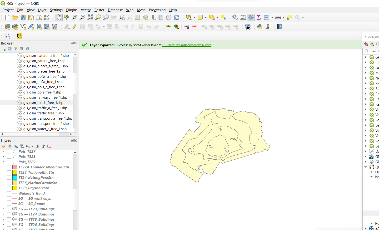
This is the result of the Iso-area generated with the Fastest path algorithm which is based on our walking speed.
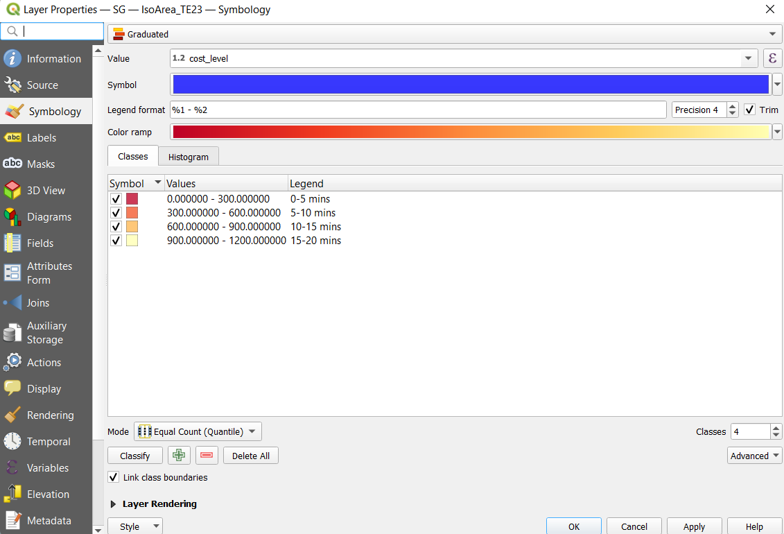

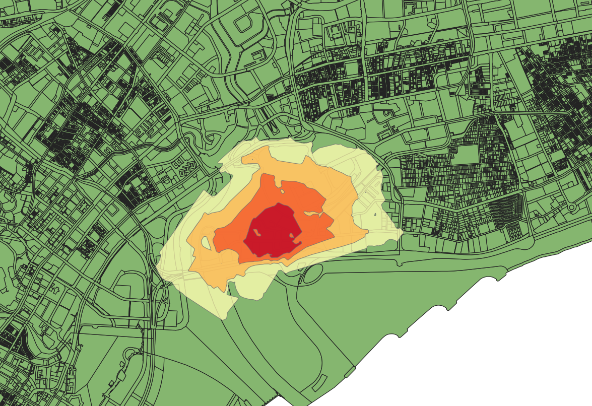
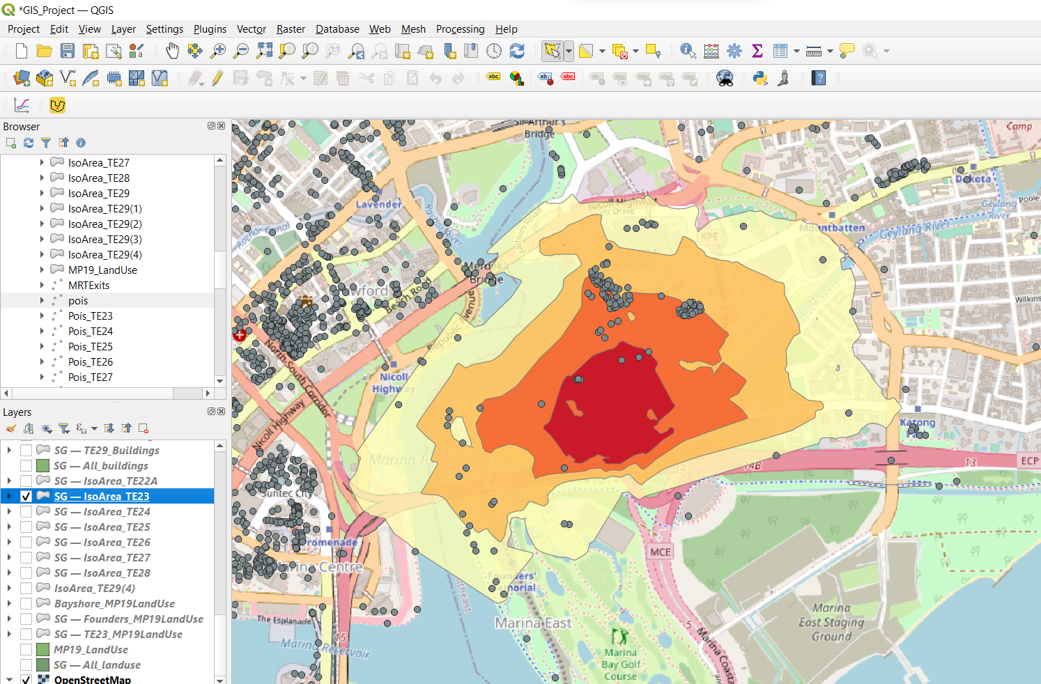
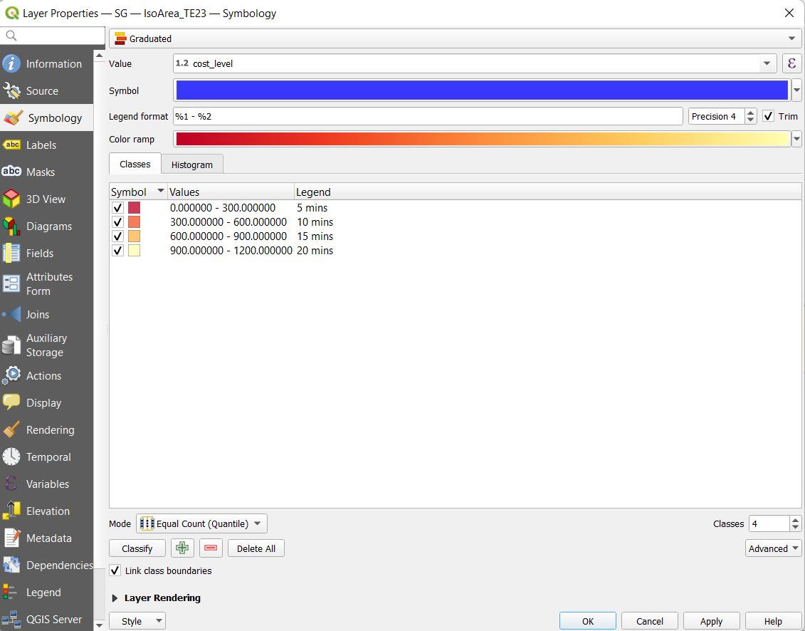
Now, we go to Symbology and classify each ring into an interval of 5 minutes, from 0 to 20 mins walking time. The red being the nearest to the MRT exit, and light yellow being the furthest.
We repeated these steps for each set of exit points from TE24 to TE29.
Identification of land use through the analysis of the Master Plan 2019 datasets
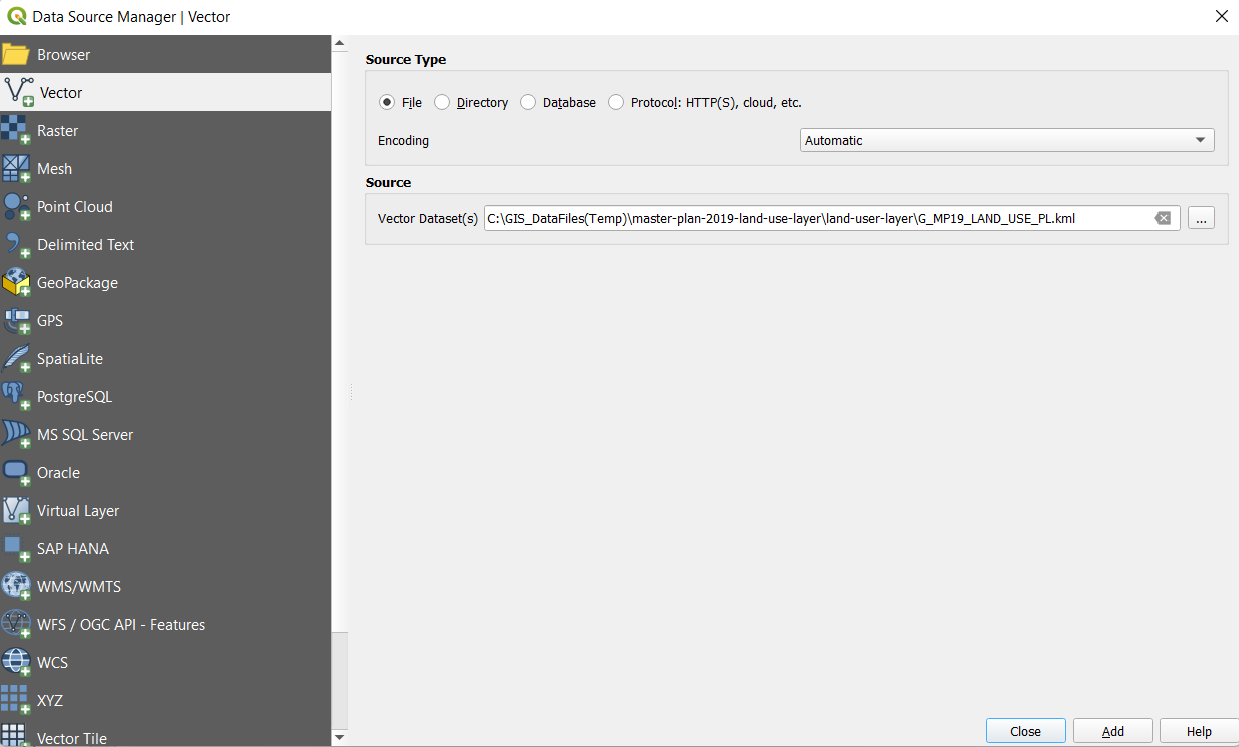
First, we opened the Master Plan 2019 Land Use KML file.
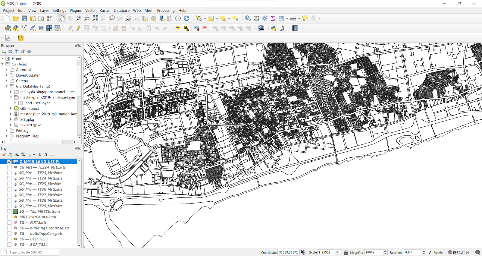
The land use layer will look like this.
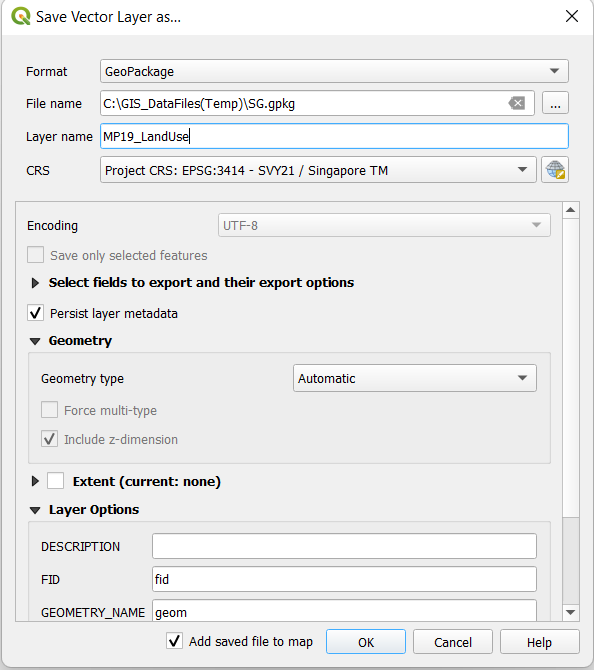
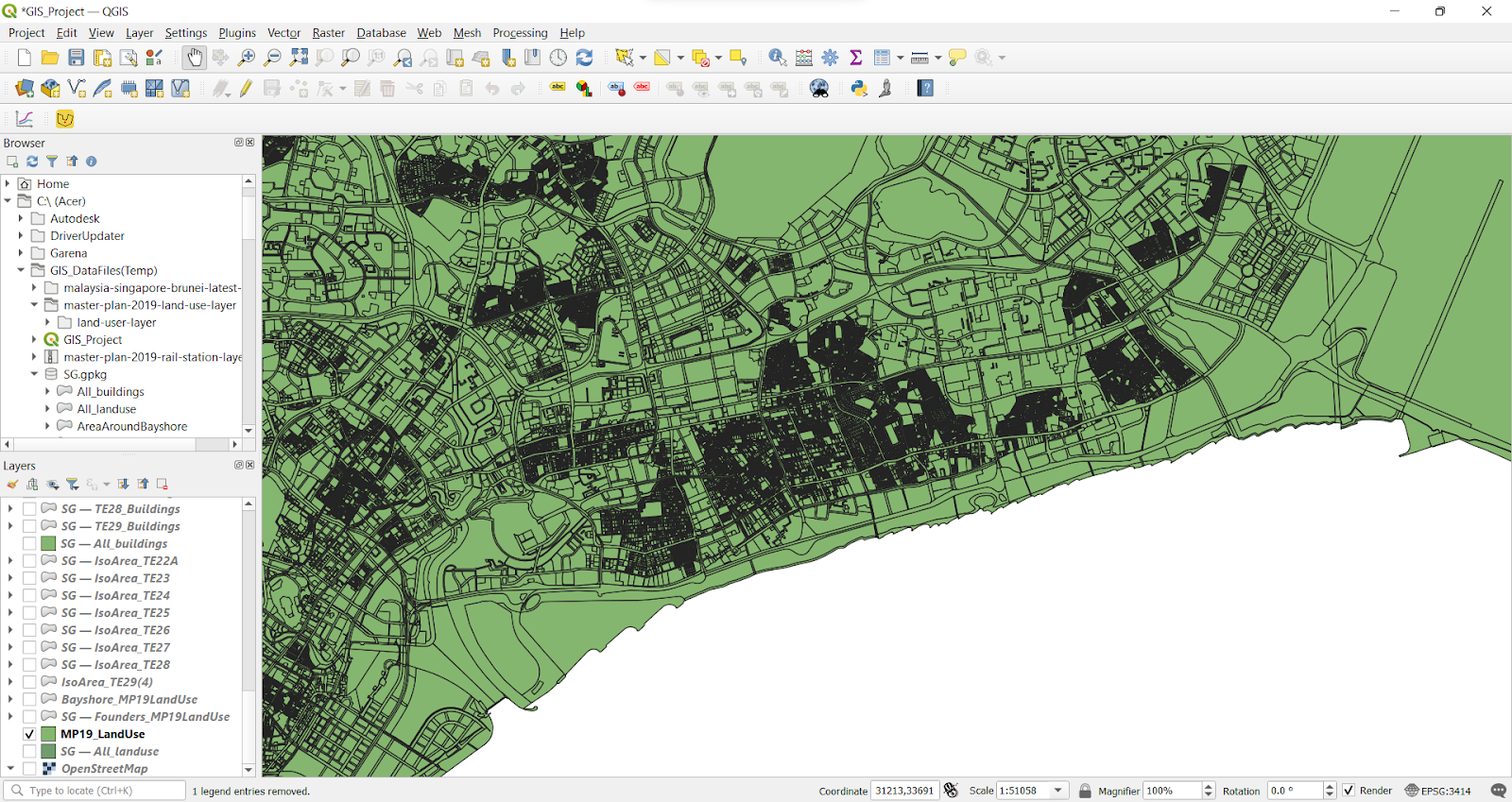
We proceeded to save it as a Geopackage file with the name “MP19_LandUse” with the appropriate Coordinate Reference System (EPSG:3414).
Toggle on the Iso-area layer and the land use area. We will be selecting the land use that intersects with the iso-area.
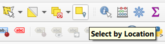
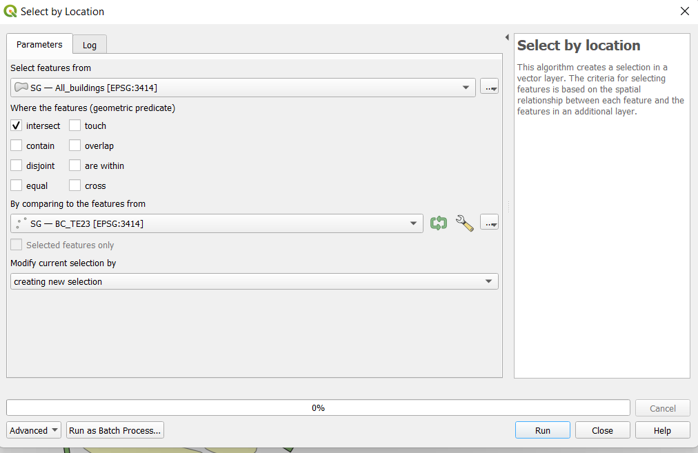
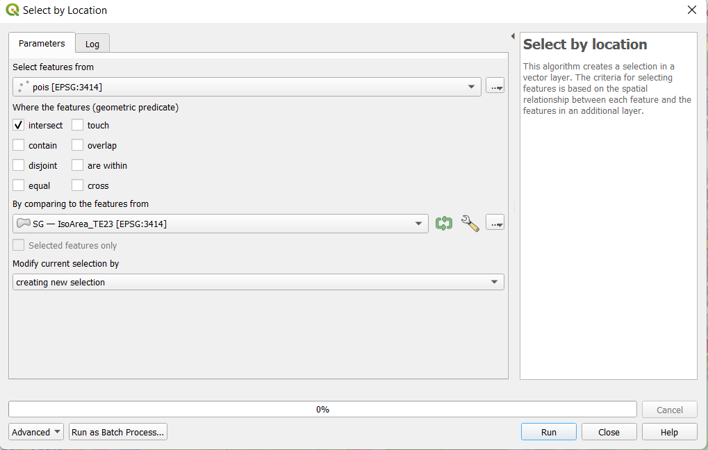
Go to the QGIS header bar and find the Select by location function.
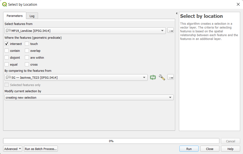
Steps:
In the Select features from column, we will choose our land use layer, which is labelled as MP19_Landuse.
Check the box beside intersect, to get the intersection between the land use layer and the iso-area.
By comparing selection by: IsoArea_TE23, which is the label for our iso-area.
We kept everything else as their default option and ran the selection.
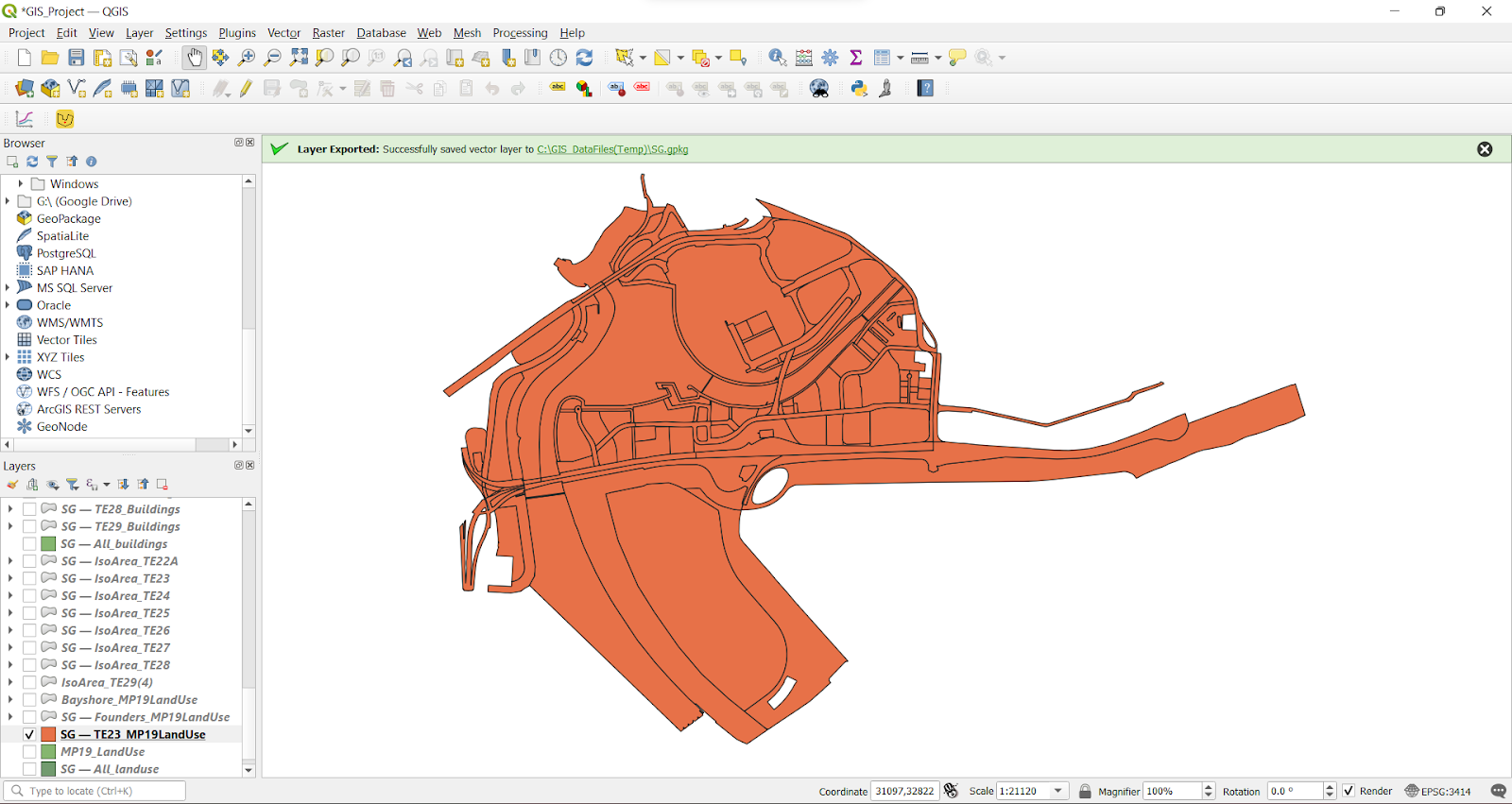
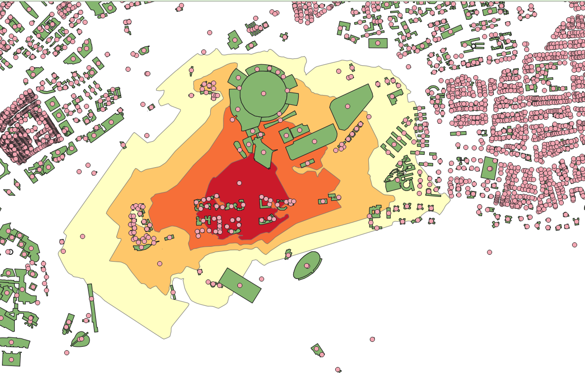
This will be the output generated, the image above shows TE23_Landuse map.
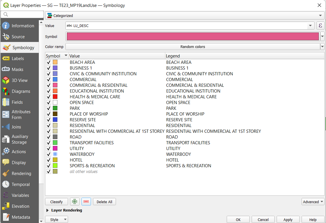
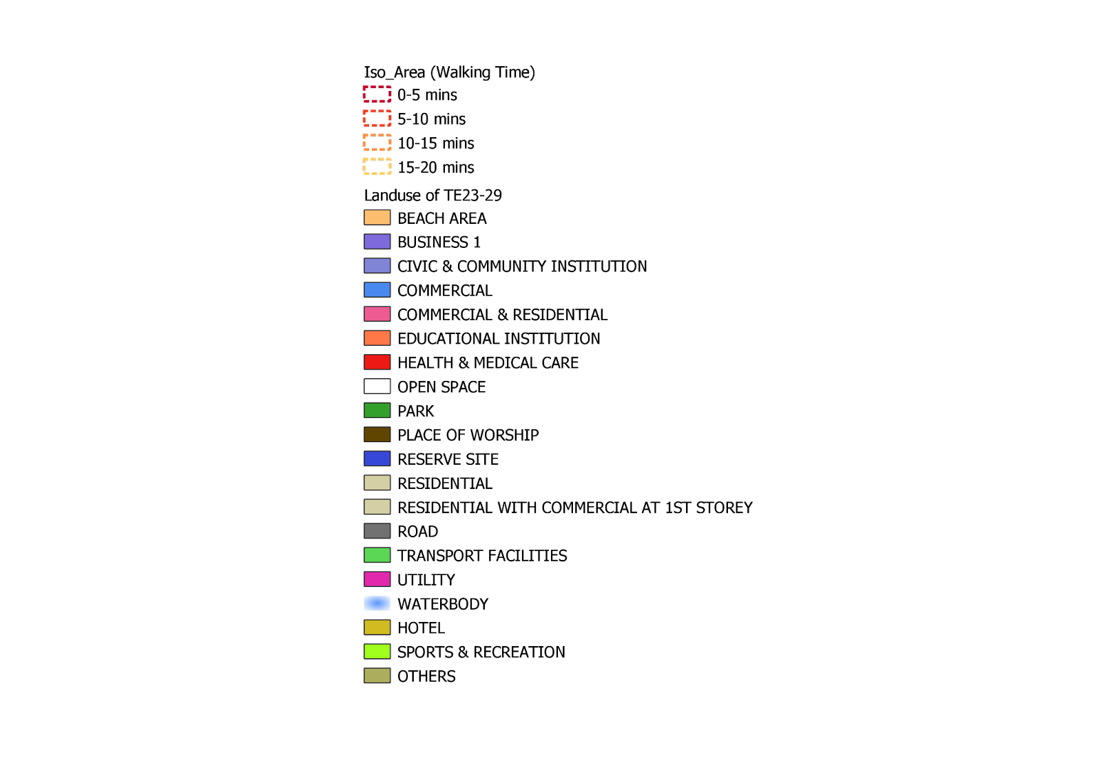
As shown in above image, we will classify the land use based on the standardised legend our team agreed on. The colours are set to be the natural colour of the landmark to make it more intuitive. Followed by saving it in a styling file.

Repeat the same steps for TE24 to TE29 landuse maps.
Generation of Centroids for Buildings
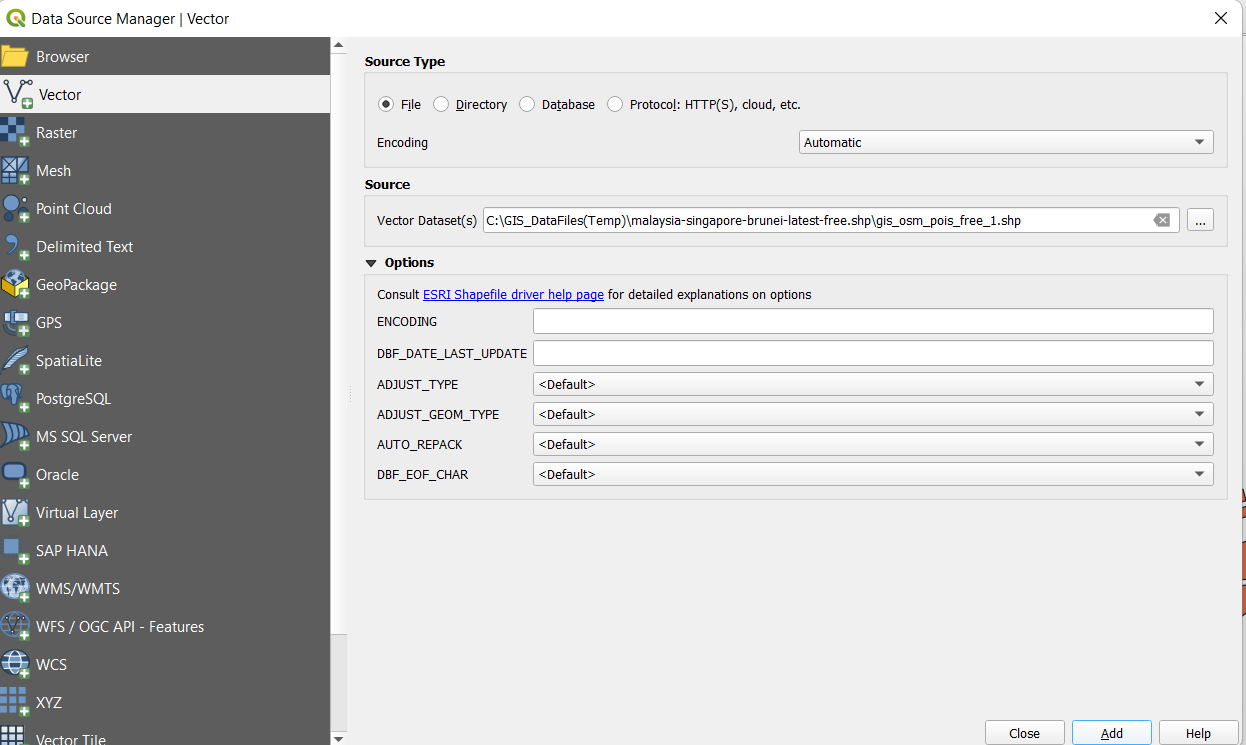
First, we opened the buildings shapefile from OpenStreetMap.
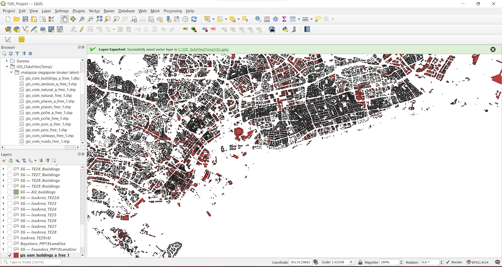
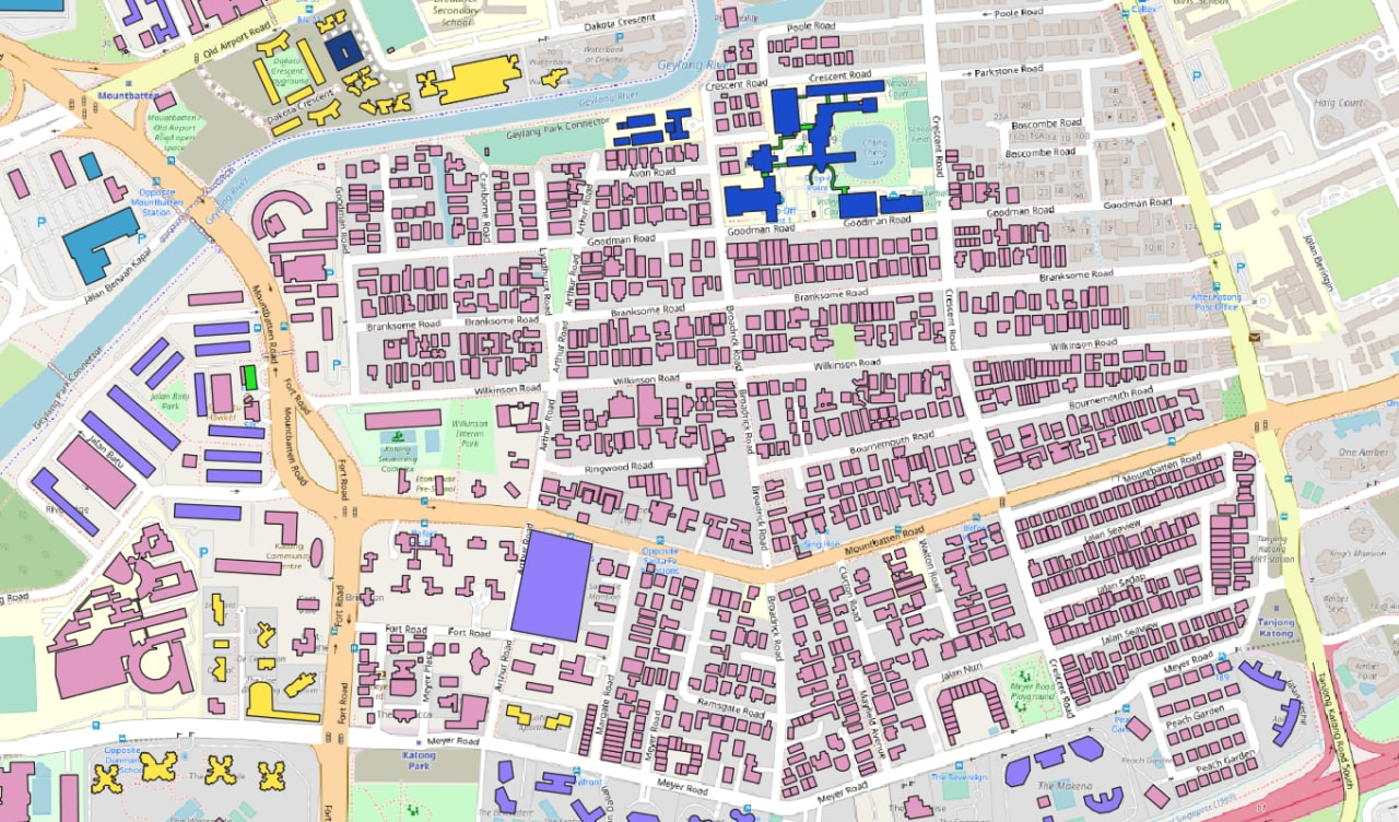
The buildings shapefile will look like this, which includes all buildings that are located in Singapore, Malaysia and Brunei. We are only interested in the buildings that are located in Singapore.
We did a selection using the Select Features by Polygon function and selected the buildings that are within the boundaries of mainland Singapore.
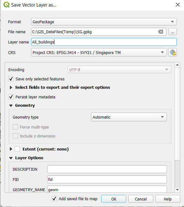
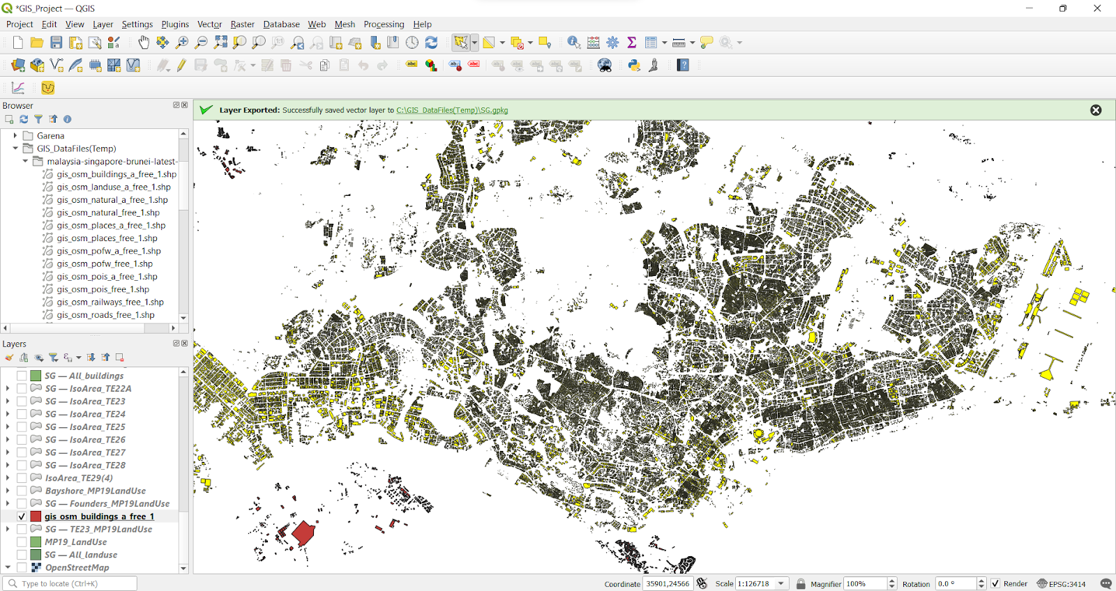
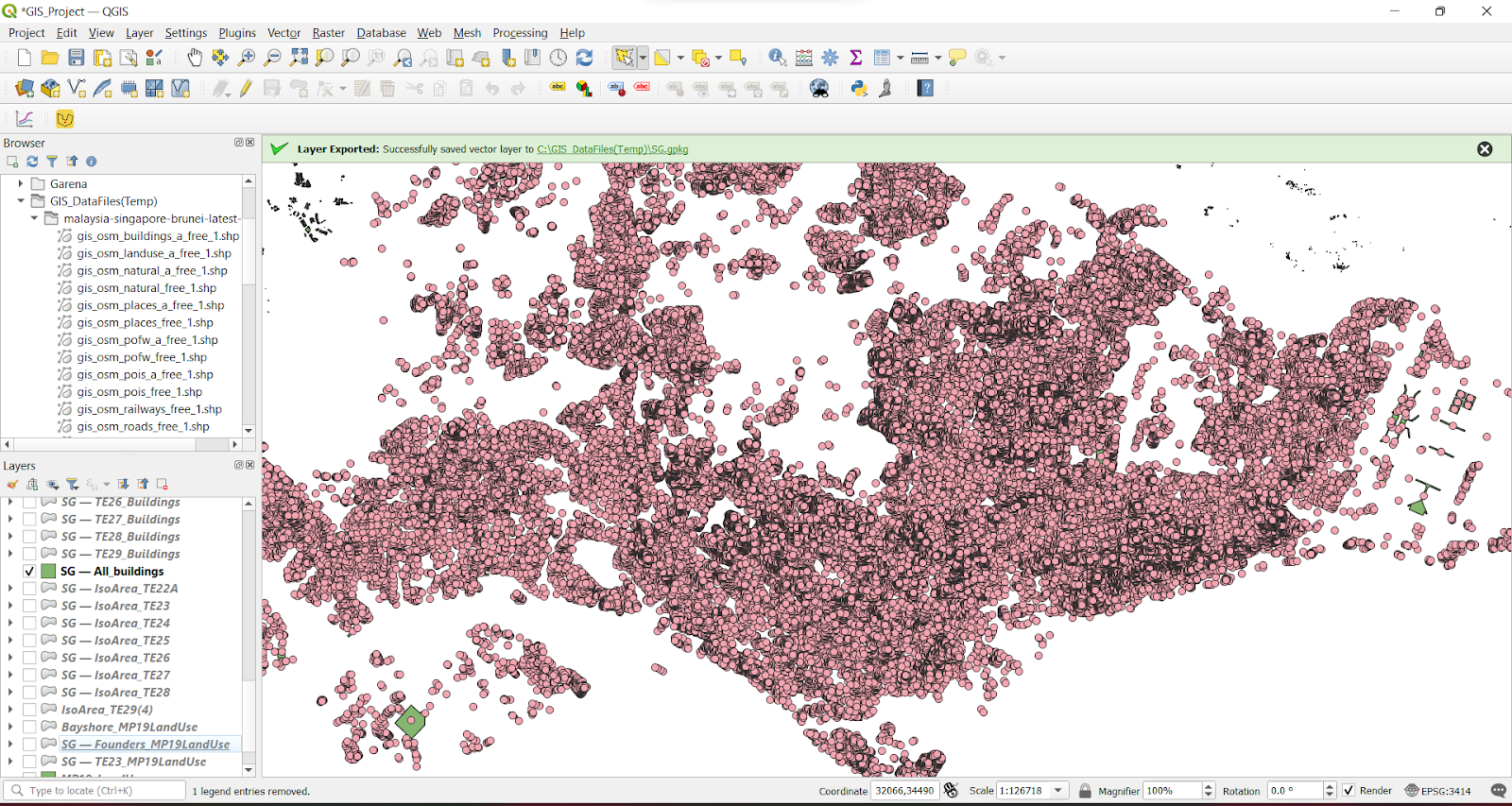
We proceeded to save it as a GeoPackage file with the label All_buildings.
’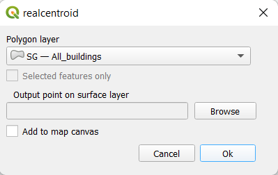
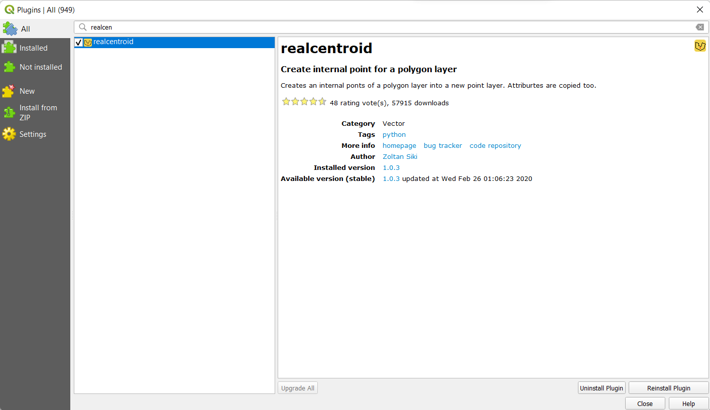
By utilising the realcentroid plugin that we downloaded separately, we were able to generate the centroids of each building. The main difference between this plugin and the built-in centroid generator is that realcentroid generates a point that is internal of a polygon, whereas the built-in one sometimes would generate a point that is external of the building polygon. We decided to use the former instead.
Picture above shows the centroids generated.
We proceeded to zoom in to the layer to get a closer look at the centroids that are within the Iso-area.
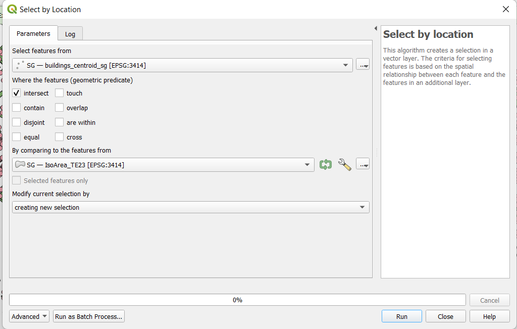
By utilizing the Select by Location function, we proceeded to select the centroids that intersect with the Iso-area.

We labelled the selected centroids as BC_TE23 and saved it as a GeoPackage file, with the correct Coordinated Reference System (EPSG:3414).
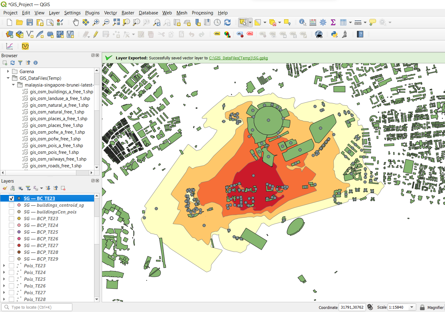
The selected centroids are marked as grey in the screenshot above. We did another selection of the buildings which intersects with the selected centroids.
Screenshot above shows the layers that are included to do this selection.
As we can see, the selected buildings are highlighted in yellow. It includes the buildings which are partly located outside the iso-area, but have their centroids located inside the Io-area.

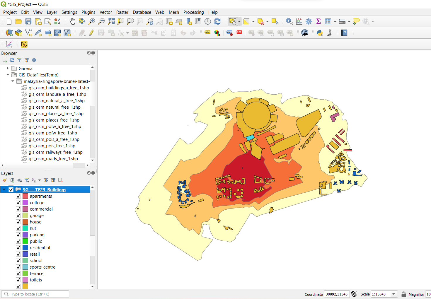
We saved these highlighted buildings as TE23_Buildings in a GeoPackage with the correct CRS.
Screenshot above shows the final result after everything is saved.
We followed these similar steps from TE24 to TE29.
Identify the types of buildings by analysing the OpenStreetMap buildings layer
We identified many null values in the attribute tables of the buildings. For example, in the picture above of TE24 buildings layer, all the pink buildings are null values. In order to fill up the null values, we placed the buildings layer over the OpenStreetMap view and compared the buildings. Some building were not identifiable through the OpenStreetMap so we took to Google to find out the specific building if it was unclear from the OpenStreetMap.

We used the Select features by freehand function to select the buildings we identified through the OpenStreetMap.
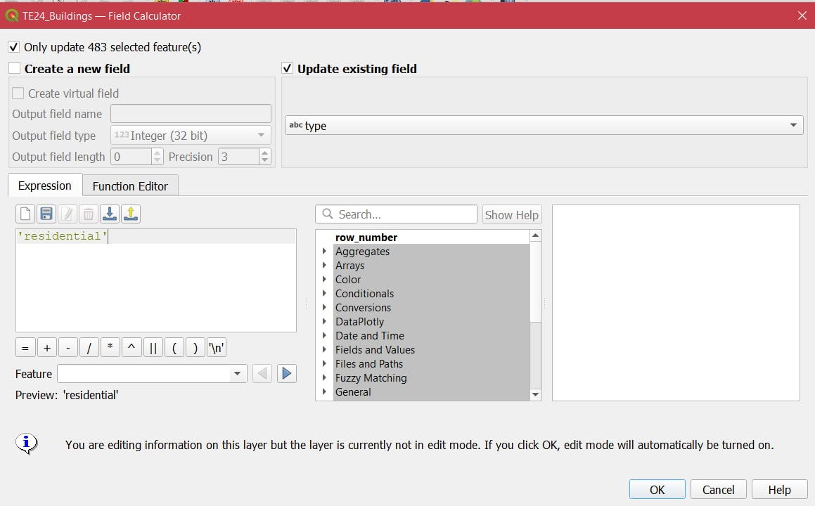
Using the Field calculator, we updated the existing field to change the null values to the appropriate categories. However, due to the large number of null values, we were unable to identify each and every building and only focused on the large areas with many null values. We also focused on picking out the buildings that would be beneficial for the residents in the area to have knowledge about such as the schools and religious places.
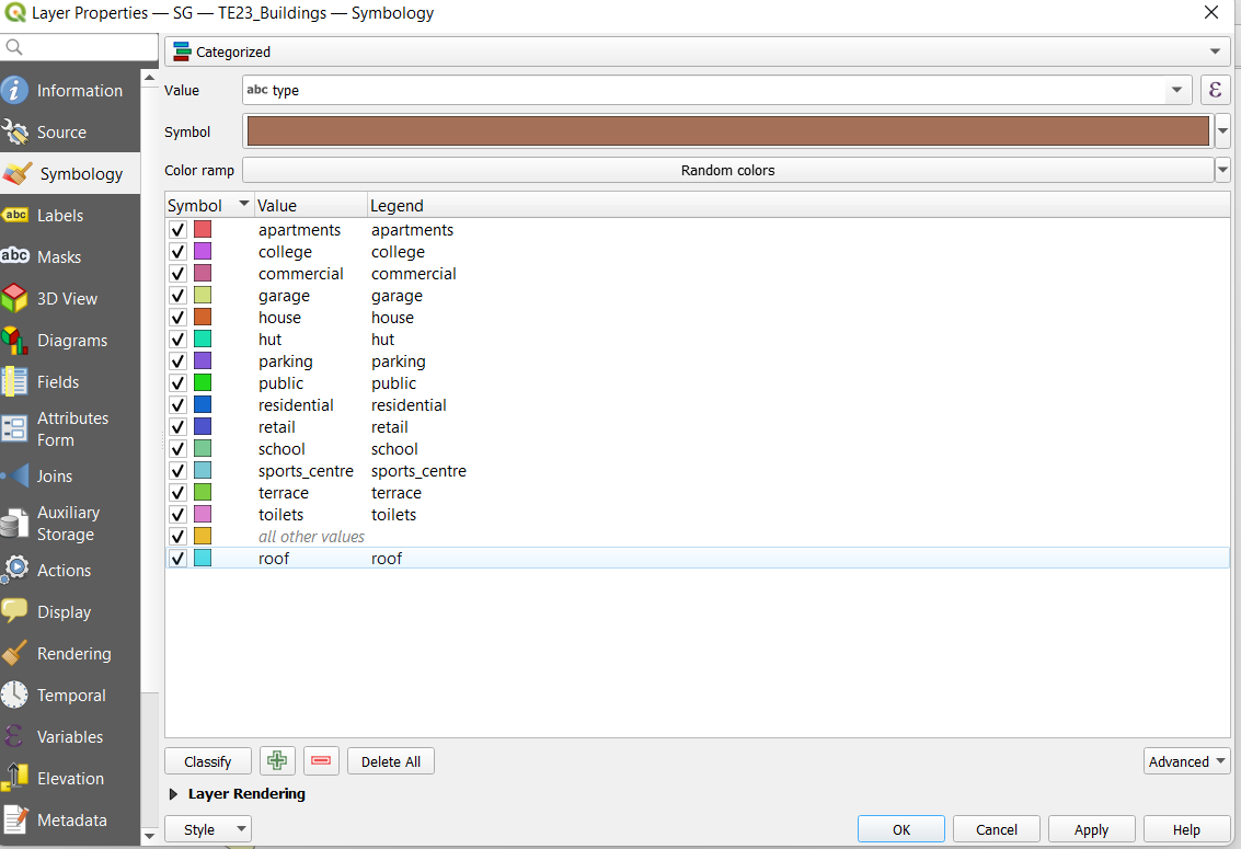
We then categorised the buildings based on colours and used the same style for each map.
Screenshot above shows the final result after categorising the buildings.
Identify the places of interest in the catchment area within the Iso-areas using the ‘Select by location’ function.
Firstly, we imported the places of interest point layer (which is labelled as POIS) into our QGIS project.
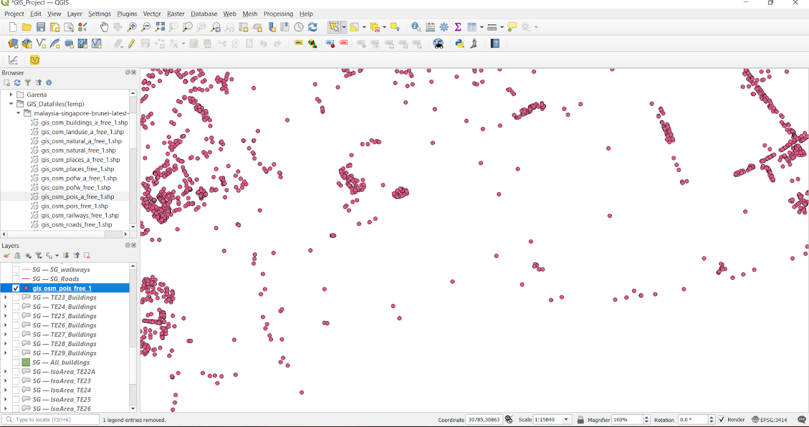
Screenshot above shows the POIS layer in its raw form.
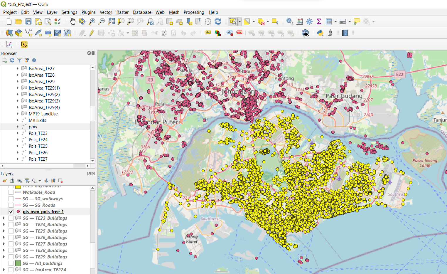
We then proceeded to select the places of interest which are located within mainland Singapore. We did this using the Select Features by Polygon function.

We then proceeded to save the selected features as a GeoPackage and assigned the appropriate CRS to the file.
By overlaying the iso-area over the map, we can see the points that are internal and external of the iso-area. We want to extract all the points of interest that are internal of the iso-area.
By using the Select by Location function, we selected all the points of interest that intersect with the iso-area.
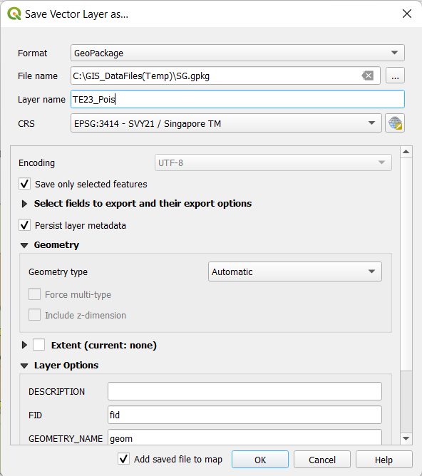
After these points of interest are selected, we then saved these selected features in a GeoPackage with the name “TE23_Pois”, indicating the points of interest that are within the iso-area of TE23 (Tanjong Rhu).
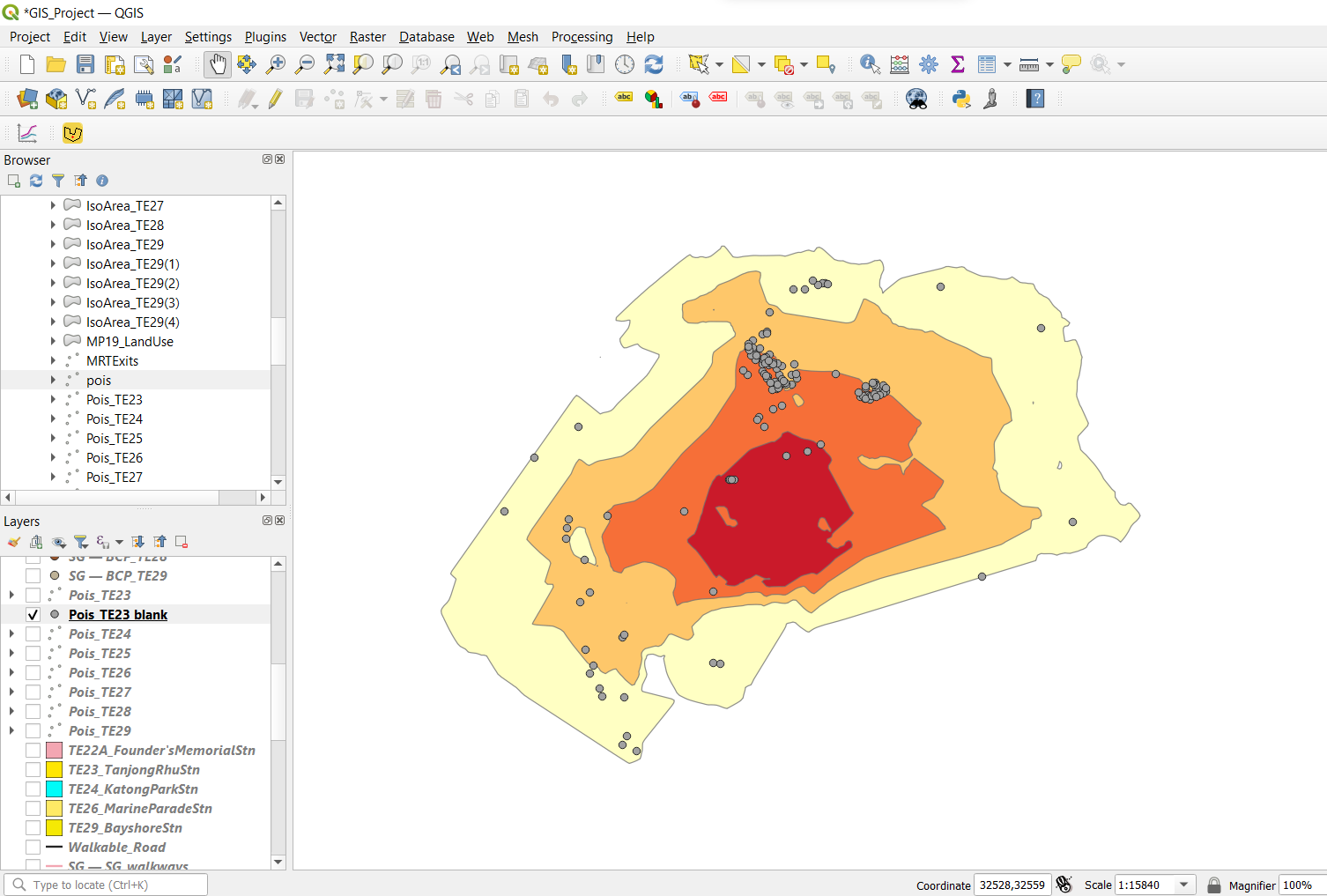
Screenshot above shows the result of our selection.
Labelling the POIS with SVG symbols, based on the type of POIS.
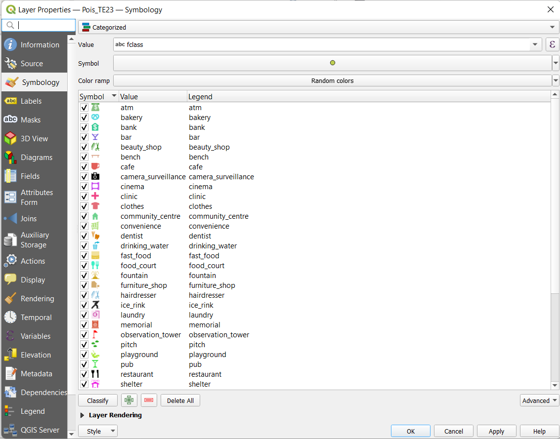
We then did a classification of these points of interest by their class (named as fclass) and assigned appropriate SVG symbols to these points. The assigning of SVG symbols were based on what the fclass is (if fclass is cafe, we assigned a logo representing a coffee cup to it).
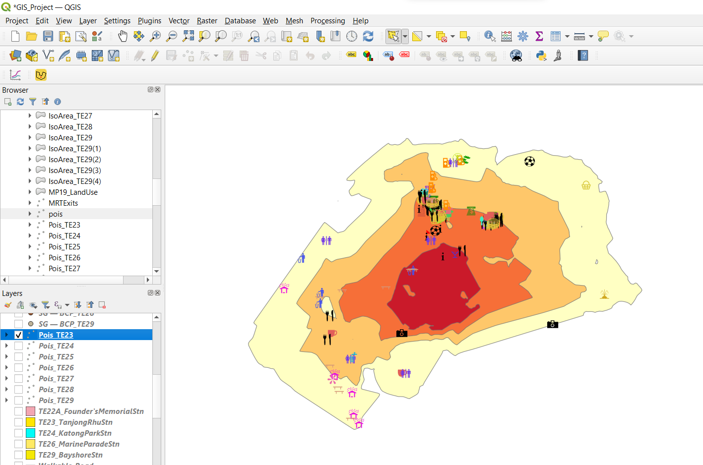
Screenshot above shows the final result of our classification and assigning of SVG symbols.
We proceeded to execute similar steps for all iso-areas from TE24 to TE29.
Standardising the symbologies for different layers
Consistency of the colours, legends and classification of our iso-areas, places of interest, buildings and land use across all MRT stations is key for intuitive understanding of our maps. Yet, it is a tedious process which requires some special tools for us to standardise the colours. Enter QGIS QML style file!
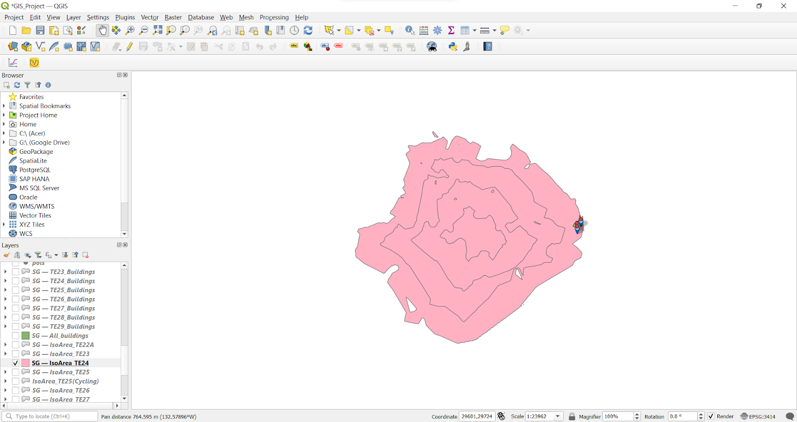
Screenshot above shows the iso-area after symbolisation is done. How do we implement these exact colours across all iso-areas?
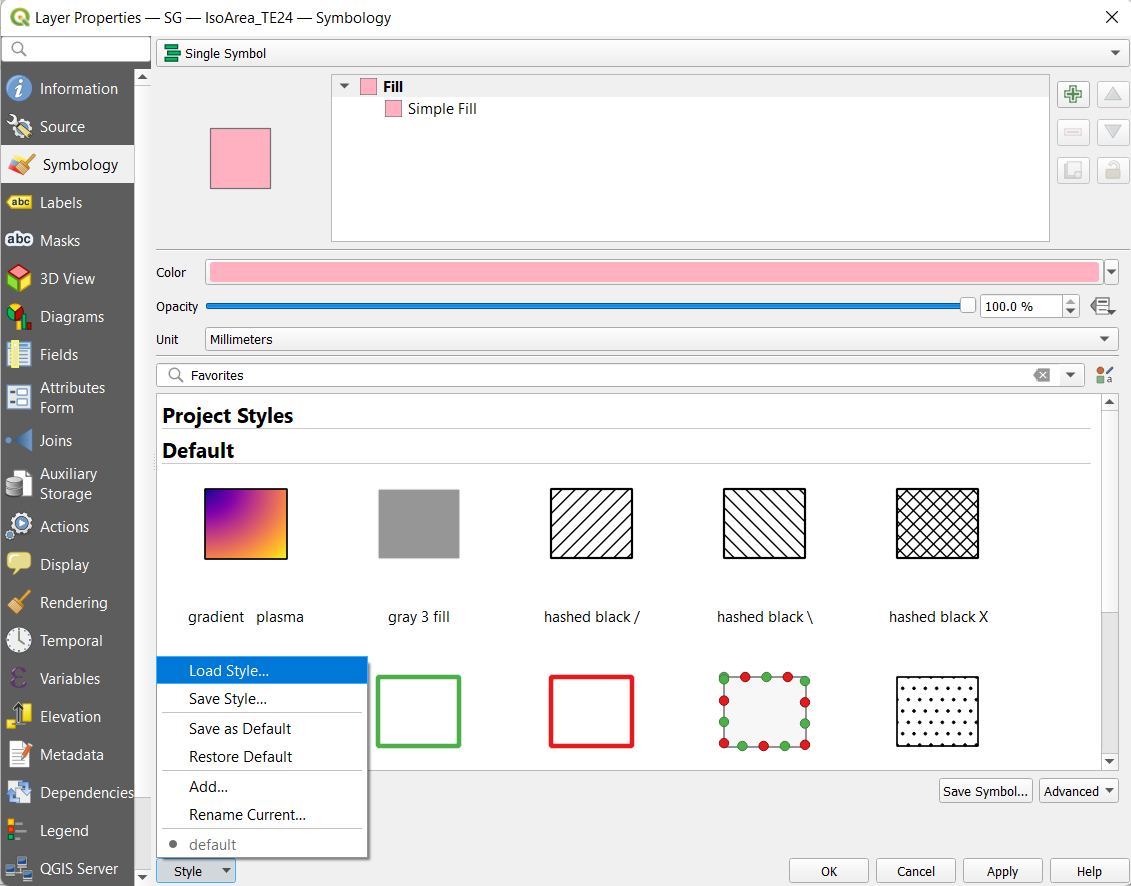
Firstly, we opened the Properties dialog window of the iso-area.
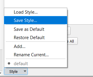
Next, we selected the Style drop-down menu and selected Save Style.
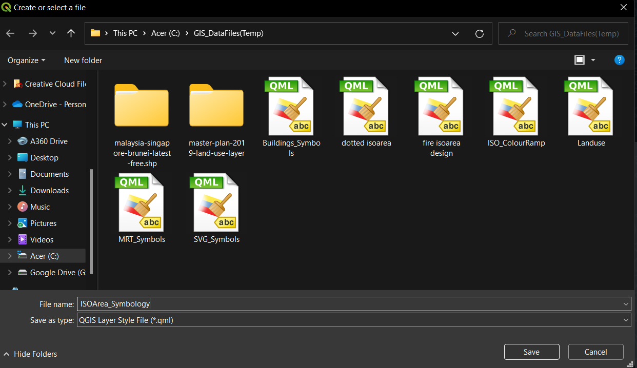
We named it according to what we are saving (in this case, an iso-area) and saved it as a QML file.
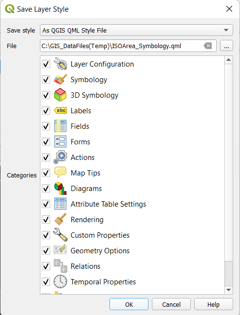
We left it in its default settings (all boxes checked) and clicked OK.
Screenshot above shows another iso-area which hasn’t been symbolised yet. Now, we want to load the qml file that we just saved to this specific iso-area.
Firstly, we opened the properties window, clicked on the Style drop-down menu and selected Load Style.
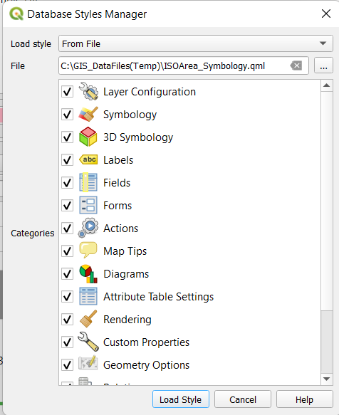
We proceeded to import the QML file that we just created (in this case, it is labelled as ISOArea_Symbology) and loaded it into this iso-area.
Screenshot above shows the result after the QML file is loaded.
We proceeded to execute the same steps for each iso-area, each set of POIS, buildings and land-use from TE24 to TE29.
Generating iso-areas for TE25 and TE28 cycling paths
The steps that we used to generate the iso-areas as shown below are similar to the iso-areas for walking paths, with a few differences. These differences are explained in detail below.
We first used the walkable paths layer that we generated earlier, as well as the MRT exits.
We then used the Iso-Area as Polygon from the QNEAT3 plugin to generate the iso-areas.
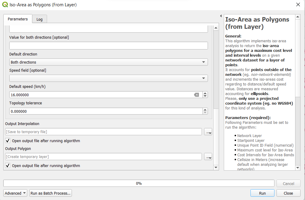
The values we inputted for the function included:
600 as the size of iso-area, which is equivalent to 600 seconds. This will be the shape of our iso-area.
16 as our default speed. This defines the average cycling speed (in km/h) in our analyses.
The rest of the values are the same as the methods we used to generate iso-areas from the walking paths, and we ran the algorithm.
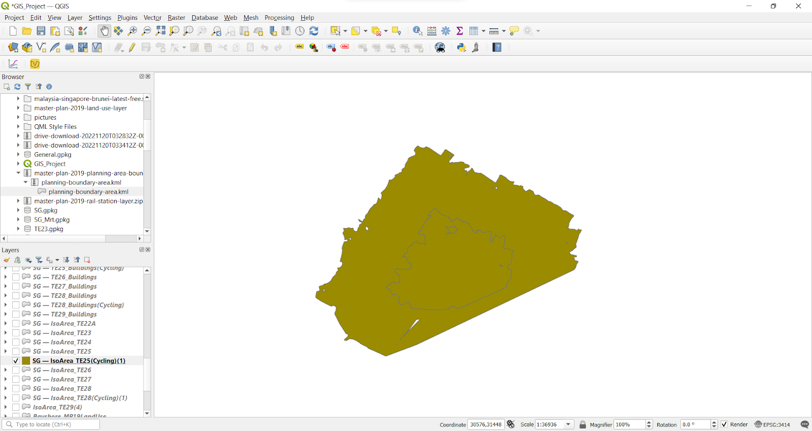 Screenshot below shows the result of running our iso-area algorithm.
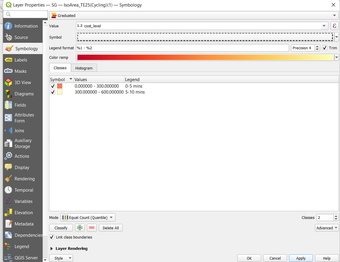
We then symbolised the layer according to its cost level (labelled as 0-5 mins and 5-10 mins respectively) and applied it to the layer.
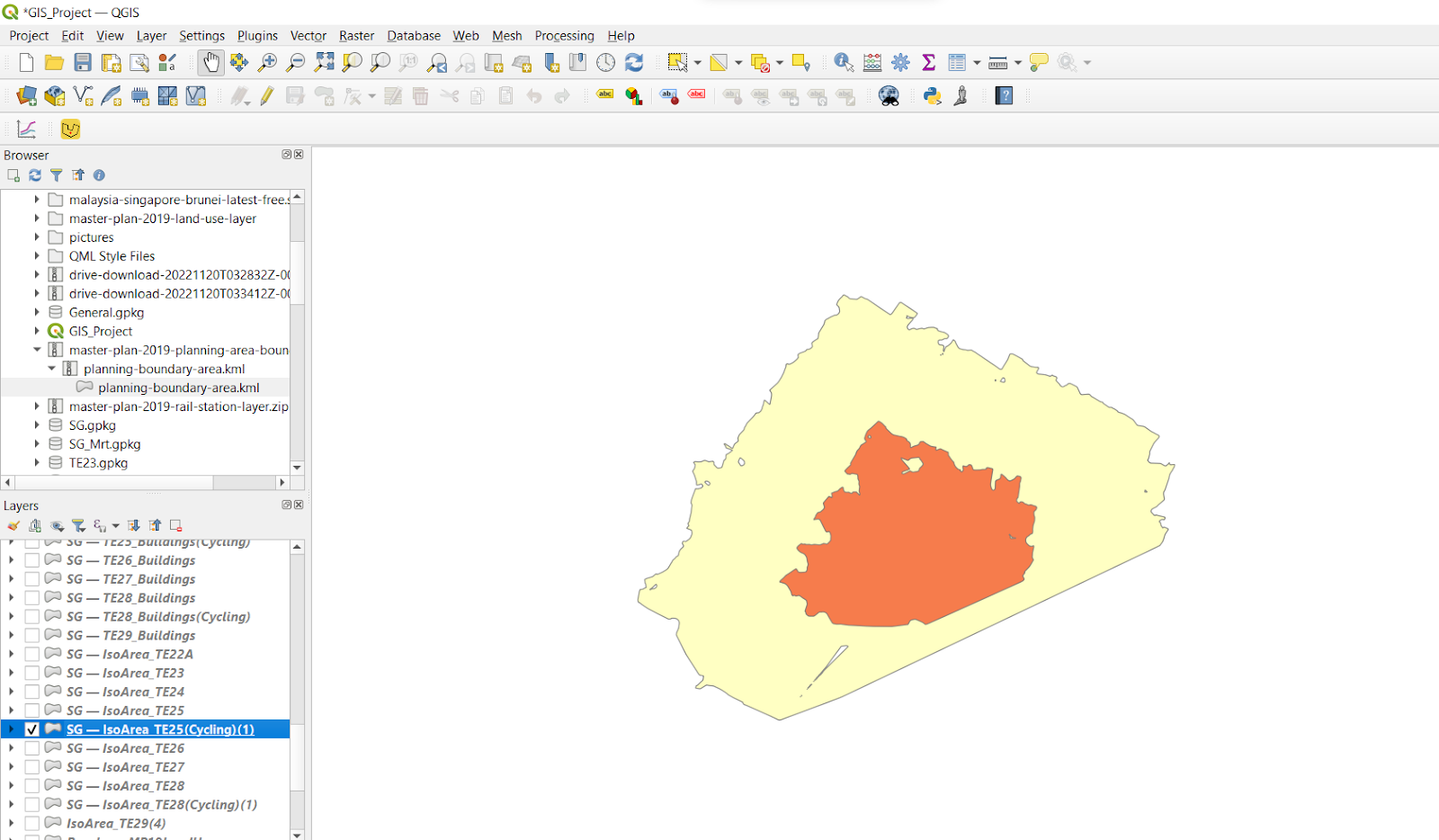
This is the final result after symbolisation.
We proceeded to do the same steps for the cycling paths of TE28.